Building a Data Warehouse with PostgreSQL, Kafka, and Debezium

---

Executive Summary

Every data team eventually hits the same wall: analytical queries running against a live transactional database. It starts small — a few dashboard queries, a couple of reports. Then one Monday morning, the engineering lead pings you: "The app is slow again."

That was the situation when I joined this project. MySQL was doing double duty — serving user transactions and powering dashboards, reverse ETL, and ELK ingestion simultaneously. The load had become a liability.

The mandate was clear: separate analytics from OLTP, keep data fresh, and don't blow the budget. What I built was a PostgreSQL-based Data Warehouse powered by Debezium CDC, Kafka, and a micro-batch stored procedure engine — a solution that could be operated by a small team, with no external cloud warehouse dependencies.

---

1. The Problem Space

Before: What Was Actually Happening

The previous architecture was a direct-read pattern:

graph LR
  MySQL[MySQL OLTP] -->|Direct Queries| ELK[ELK Stack]
  MySQL -->|Direct Queries| Dashboards[BI Dashboards]
  MySQL -->|Direct Sync| RevETL[Reverse ETL Systems]

Every dashboard refresh, every Kibana aggregation, every reverse ETL sync was hitting the same MySQL instance that was handling live user writes. This created three hard problems:

1. OLTP Performance Degradation Analytical queries on MySQL are fundamentally different from OLTP queries — they scan large ranges, perform aggregations, and hold table-level read locks longer. Under moderate analytical load, INSERT and UPDATE latency on the application side climbed noticeably.

2. No Historical Layer MySQL is an OLTP store — it's designed for current state, not history. There was no slowly changing dimension (SCD) tracking, no point-in-time query support, no ability to audit how a record looked on a specific date.

3. Scattered Business Logic Transformation rules were duplicated across the ELK index mappings, the BI tool's calculated fields, and reverse ETL sync scripts. When a business rule changed, it had to be patched in three places — each with a different query language.

The Constraints That Shaped Every Decision

Constraint	Implication
Zero impact on OLTP writes	No synchronous triggers, no read replicas for writes
Budget: near-zero additional infrastructure	No Snowflake, no BigQuery, no Spark cluster
Latency: <5 min for reverse ETL	Near real-time ingestion required
Small team, SQL-native	Complex orchestration tools (Airflow) are out
Must be backfill-safe	Every job must be safely re-runnable

---

2. Architecture Design

The Core Principle: Decouple Capture from Transformation

The architecture separates responsibilities into two independent concerns:

1. Ingestion Layer: MySQL → Debezium → Kafka → PostgreSQL raw schema (event-driven, near real-time)
2. Transformation Layer: raw → staging → core → datamart (SQL stored procedures, scheduled via pg_cron)

This separation means ingestion is never blocked by transformation, and transformation can safely lag behind ingestion without losing any events.

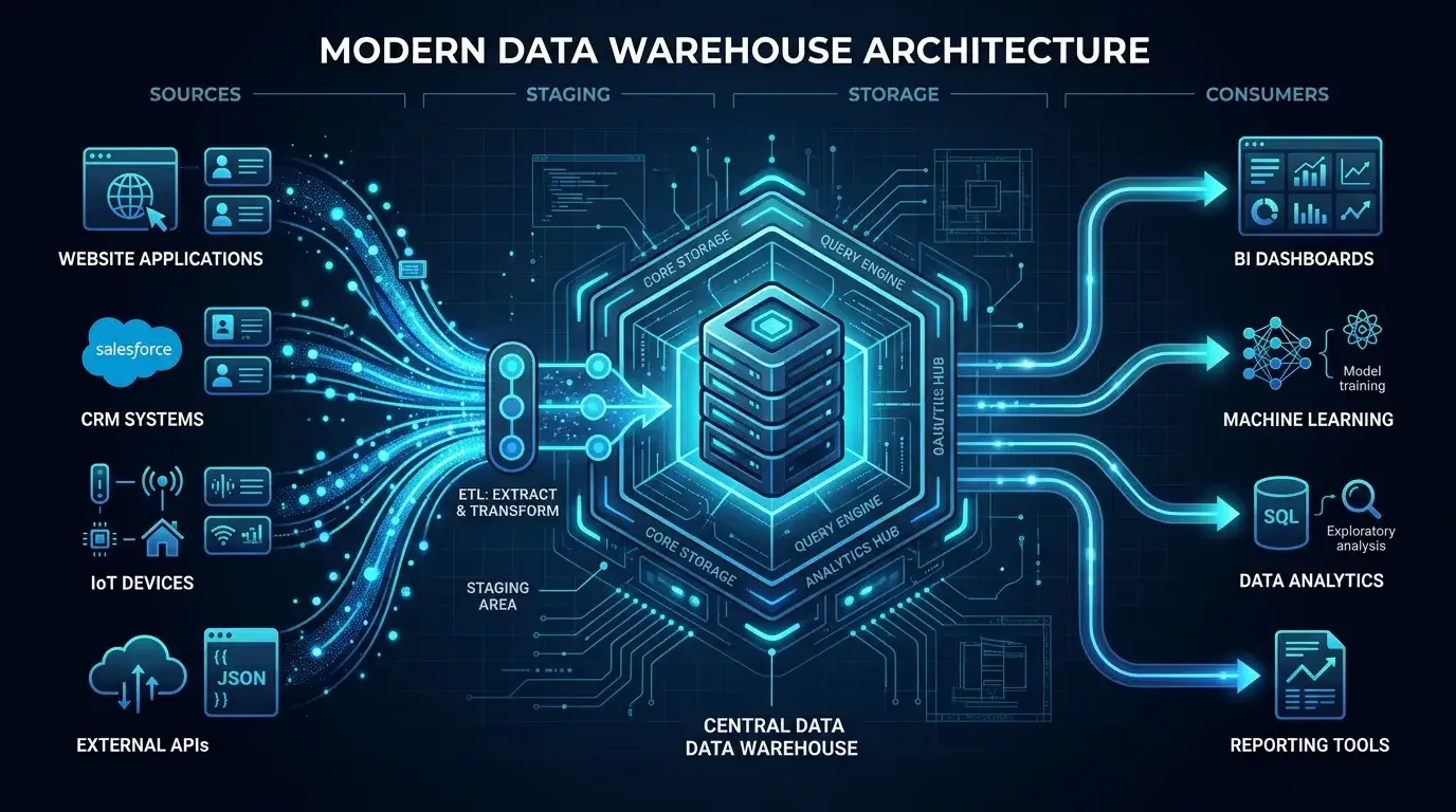
graph TD
  subgraph Source
    MySQL[MySQL OLTP\nApplication DB]
  end

  subgraph Ingestion
    Debezium[Debezium\nMySQL Connector]
    Kafka[Apache Kafka\nEvent Buffer]
    Consumer[Kafka Consumer\nUpsert Worker]
  end

  subgraph DWH["PostgreSQL Data Warehouse"]
    Raw[(raw.*\nCDC Sink)]
    Staging[(staging.*\nCleaned & Typed)]
    Core[(core.*\nFacts & Dims)]
    Datamart[(datamart.*\nPre-aggregated)]
  end

  subgraph Consumers
    BI[BI Dashboards]
    RevETL[Reverse ETL]
    ELK[ELK Stack]
  end

  MySQL -->|Binlog CDC| Debezium
  Debezium -->|CDC Events| Kafka
  Kafka --> Consumer
  Consumer -->|UPSERT| Raw
  Raw -->|pg_cron trigger| Staging
  Staging -->|pg_cron trigger| Core
  Core -->|pg_cron trigger| Datamart
  Datamart --> BI
  Datamart --> RevETL
  Datamart --> ELK

Why PostgreSQL as the Warehouse?

This choice raised eyebrows internally. PostgreSQL is an OLTP database — why not a proper columnar store like Redshift or Snowflake?

The reasoning was deliberate:

• The team already knew SQL on MySQL. Switching to PostgreSQL was a minor cognitive jump. Switching to Redshift SQL, BigQuery's dialect, or Spark's DataFrame API would have been major.
• The data volumes were manageable. I wasn't processing petabytes. With proper partitioning, indexing, and VACUUM, PostgreSQL handles hundreds of millions of rows comfortably for our query patterns.
• Window functions, materialized views, and partitioning. PostgreSQL's analytical feature set is genuinely excellent for moderate-scale DWH use.
• No additional managed service cost. The PostgreSQL instance ran on infrastructure we already had.

The tradeoff was that PostgreSQL requires more active tuning than a managed warehouse. I accepted that and built the maintenance routines into the platform.

---

3. The Ingestion Layer: CDC with Debezium + Kafka

How Change Data Capture Works Here

MySQL has a binary log (binlog) — a sequential record of every write that occurs. Debezium's MySQL connector tails this binlog and converts each INSERT, UPDATE, and DELETE into a structured CDC event published to Kafka.

This approach has a critical advantage over polling: it captures every row state, not just the latest one. A polling approach reading WHERE updated_at > last_run will miss records that were updated and deleted between runs. CDC doesn't have this gap.

Debezium Configuration Decisions

A few non-obvious configuration decisions that mattered in practice:

Snapshot Mode: initial On first startup, Debezium takes a consistent snapshot of the entire table before switching to binlog tailing. I configured snapshot.mode=initial so the raw schema starts with a complete baseline.

Tombstone Events Debezium publishes a tombstone (null-value) message after a delete event. This is important for Kafka log compaction — without it, deleted records pile up in the compacted log. I set tombstones.on.delete=true.

Decimal Handling MySQL DECIMAL types were configured with decimal.handling.mode=double to avoid schema evolution headaches with Avro serialization of arbitrary-precision types.

The Kafka Consumer: Upsert Into Raw

The Kafka consumer reads CDC events and applies them to the raw schema in PostgreSQL as UPSERT (INSERT ON CONFLICT DO UPDATE) operations.

The raw schema tables mirror the MySQL source schema almost exactly, with two additions:

-- Every raw table has these two metadata columns
_cdc_deleted_at   TIMESTAMPTZ   -- populated from Debezium delete events
_cdc_updated_at   TIMESTAMPTZ   -- populated from Debezium event timestamp

The upsert pattern:

INSERT INTO raw.orders (id, user_id, status, total, created_at, _cdc_updated_at)
VALUES ($1, $2, $3, $4, $5, NOW())
ON CONFLICT (id) DO UPDATE SET
  user_id      = EXCLUDED.user_id,
  status       = EXCLUDED.status,
  total        = EXCLUDED.total,
  _cdc_updated_at = EXCLUDED._cdc_updated_at;

Deletes from MySQL result in the row being retained in raw with _cdc_deleted_at populated — we don't physically delete from the warehouse. Downstream layers filter out logically deleted records as needed.

---

4. Data Modeling: The Four-Layer Schema

Each schema layer has a single, well-defined responsibility. This makes the data lineage auditable and transformations testable in isolation.

Layer 1 — raw.*: The Immutable Source Mirror

Raw is a nearly 1:1 copy of MySQL, augmented with CDC metadata. No business logic lives here. The only transformations are:

• Type coercion for PostgreSQL compatibility (e.g., MySQL tinyint(1) → PostgreSQL boolean)
• Addition of _cdc_deleted_at and _cdc_updated_at metadata columns

No data is ever deleted from raw. It's the system of record within the DWH.

Layer 2 — staging.*: Cleansed & Validated

Staging performs the dirty work:

• Deduplication: handles race conditions where two CDC events arrive for the same record in the same micro-batch
• Type casting: parses string timestamps into proper TIMESTAMPTZ, normalizes phone number formats, etc.
• Null handling: replaces known sentinel nulls (e.g., 'N/A', '0000-00-00') with proper NULL
• Filtering: excludes logically deleted records (WHERE _cdc_deleted_at IS NULL)

Layer 3 — core.*: Business-Modeled Facts & Dimensions

Core implements the actual data model. I used a Kimball-style star schema — not because it's a religion, but because the query patterns and the team's familiarity with SQL JOIN made it the pragmatic choice.

core.fact_orders
  ├── order_id (PK)
  ├── user_dim_key (FK → core.dim_users)
  ├── product_dim_key (FK → core.dim_products)
  ├── order_date_key (FK → core.dim_date)
  ├── status
  ├── gross_revenue
  ├── net_revenue
  └── _etl_batch_id

core.dim_users (SCD Type 2)
  ├── user_dim_key (surrogate PK)
  ├── user_id (natural key)
  ├── full_name, email, tier
  ├── valid_from, valid_to
  └── is_current

SCD Type 2 for users and products. When a user's tier changes, I close the current record (set valid_to, is_current = false) and insert a new record. This enables point-in-time analysis — "what tier was this user when they placed this order?"

Layer 4 — datamart.*: Pre-aggregated for Consumers

Dashboards and reverse ETL read from datamart tables, not from core. These are pre-aggregated and indexed specifically for their consumer's access patterns:

-- Example: daily revenue datamart for BI dashboards
CREATE TABLE datamart.daily_revenue AS
SELECT
  d.date                     AS report_date,
  u.tier                     AS user_tier,
  p.category                 AS product_category,
  SUM(o.gross_revenue)       AS gross_revenue,
  SUM(o.net_revenue)         AS net_revenue,
  COUNT(DISTINCT o.order_id) AS order_count,
  COUNT(DISTINCT o.user_dim_key) AS unique_buyers
FROM core.fact_orders o
JOIN core.dim_date d    ON o.order_date_key  = d.date_key
JOIN core.dim_users u   ON o.user_dim_key    = u.user_dim_key AND u.is_current
JOIN core.dim_products p ON o.product_dim_key = p.product_dim_key AND p.is_current
GROUP BY 1, 2, 3;

The BI team reads datamart.daily_revenue. They never write SQL against core or raw.

---

5. The Transformation Engine: Stored Procedures + pg_cron

Why Stored Procedures?

The alternative was a Python-based orchestration layer (Airflow DAGs calling pandas transforms). I rejected it for this project for pragmatic reasons:

1. All the data is already in PostgreSQL. Moving it out to Python for transformation and back in is wasteful I/O.
2. Set-based SQL transforms outperform row-by-row Python at these volumes by orders of magnitude.
3. The team writes SQL every day. Debugging a stored procedure is much faster for them than debugging a pandas pipeline.

The stored procedures follow a consistent interface:

CREATE OR REPLACE PROCEDURE etl.process_orders(
  p_business_date    DATE,
  p_start_ts         TIMESTAMPTZ,
  p_end_ts           TIMESTAMPTZ
)
LANGUAGE plpgsql
AS $$
DECLARE
  v_batch_id   BIGINT;
  v_rows_in    INT := 0;
  v_rows_out   INT := 0;
BEGIN
  -- 1. Open a batch control record
  INSERT INTO etl.job_runs (job_name, started_at, status, p_business_date, p_start_ts, p_end_ts)
  VALUES ('process_orders', NOW(), 'running', p_business_date, p_start_ts, p_end_ts)
  RETURNING id INTO v_batch_id;

  -- 2. Stage: clean and deduplicate
  INSERT INTO staging.orders (...)
  SELECT DISTINCT ON (id) ...
  FROM raw.orders
  WHERE _cdc_updated_at BETWEEN p_start_ts AND p_end_ts
    AND _cdc_deleted_at IS NULL
  ORDER BY id, _cdc_updated_at DESC;

  GET DIAGNOSTICS v_rows_in = ROW_COUNT;

  -- 3. Core: merge into fact table
  INSERT INTO core.fact_orders (...)
  SELECT ... FROM staging.orders WHERE batch_id = v_batch_id
  ON CONFLICT (order_id) DO UPDATE SET
    status       = EXCLUDED.status,
    net_revenue  = EXCLUDED.net_revenue,
    _etl_batch_id = EXCLUDED._etl_batch_id;

  GET DIAGNOSTICS v_rows_out = ROW_COUNT;

  -- 4. Refresh the datamart
  CALL etl.refresh_datamart_daily_revenue(p_business_date);

  -- 5. Close the batch as succeeded
  UPDATE etl.job_runs
  SET status = 'succeeded', finished_at = NOW(),
      rows_in = v_rows_in, rows_out = v_rows_out
  WHERE id = v_batch_id;

EXCEPTION WHEN OTHERS THEN
  UPDATE etl.job_runs
  SET status = 'failed', finished_at = NOW(), error_message = SQLERRM
  WHERE id = v_batch_id;
  RAISE;
END;
$$;

Idempotency Is Non-Negotiable

Every procedure is designed to be safely re-runnable for the same parameters. If a job fails and is retried for the same time window, the final state in the warehouse must be identical to what a successful first run would have produced.

This is enforced by the INSERT ... ON CONFLICT DO UPDATE pattern throughout. There are no unconditional INSERT INTO ... SELECT statements — everything is upserted.

Watermarking for Near Real-Time Reverse ETL

The micro-batch procedures that feed reverse ETL systems run every 1–5 minutes. The watermark logic prevents data loss while avoiding redundant processing:

CREATE OR REPLACE PROCEDURE etl.process_orders_micro_batch()
LANGUAGE plpgsql AS $$
DECLARE
  v_last_watermark  TIMESTAMPTZ;
  v_upper_bound     TIMESTAMPTZ;
  v_overlap_window  INTERVAL := '2 minutes';
BEGIN
  -- Get the end_time of the last successful run as our watermark
  SELECT end_ts INTO v_last_watermark
  FROM etl.job_runs
  WHERE job_name = 'process_orders_micro_batch'
    AND status   = 'succeeded'
  ORDER BY finished_at DESC
  LIMIT 1;

  -- Default to 24 hours ago if no prior run exists
  v_last_watermark := COALESCE(v_last_watermark, NOW() - INTERVAL '24 hours');

  -- Upper bound is set at procedure start (not end)
  v_upper_bound := NOW();

  -- Read from (watermark - overlap) to catch late-arriving data
  CALL etl.process_orders(
    p_business_date => v_upper_bound::DATE,
    p_start_ts      => v_last_watermark - v_overlap_window,
    p_end_ts        => v_upper_bound
  );
END;
$$;

The overlap window (2 minutes) is intentional. It re-reads records from slightly before the last watermark to handle two scenarios:

1. Late-arriving CDC events: Kafka occasionally delivers events slightly out of order.
2. Identical updated_at timestamps: Records updated in the same second as the previous watermark boundary need to be captured.

Because the upsert is idempotent, re-reading records from the overlap window has no adverse effect on data correctness.

pg_cron Scheduling

-- Micro-batch for reverse ETL: every 5 minutes
SELECT cron.schedule('orders-micro-batch', '*/5 * * * *',
  $$CALL etl.process_orders_micro_batch()$$);

-- Daily batch for KPIs: 1 AM every day
SELECT cron.schedule('orders-daily', '0 1 * * *',
  $$CALL etl.process_orders(CURRENT_DATE - 1, NULL, NULL)$$);

-- Weekly trend batch: Sunday 2 AM
SELECT cron.schedule('orders-weekly', '0 2 * * 0',
  $$CALL etl.process_weekly_trends(DATE_TRUNC('week', CURRENT_DATE - 7))$$);

pg_cron.job_run_details gives us a queryable history of every execution — job name, scheduled time, start time, end time, and return status — without any external monitoring infrastructure.

---

6. Data Quality & Operational Observability

The Control Table

Every job run writes to etl.job_runs:

CREATE TABLE etl.job_runs (
  id               BIGSERIAL PRIMARY KEY,
  job_name         TEXT          NOT NULL,
  started_at       TIMESTAMPTZ   NOT NULL DEFAULT NOW(),
  finished_at      TIMESTAMPTZ,
  status           TEXT          CHECK (status IN ('running', 'succeeded', 'failed')),
  p_business_date  DATE,
  p_start_ts       TIMESTAMPTZ,
  p_end_ts         TIMESTAMPTZ,
  rows_in          INT,
  rows_out         INT,
  error_message    TEXT
);

This table is the first stop for any data freshness question. A simple query tells us when each job last ran, how many rows it processed, and whether it succeeded.

Automated Data Quality Checks

A suite of SQL assertions runs after each daily batch:

-- Freshness check: did we process data for the expected date?
DO $$
BEGIN
  ASSERT (
    SELECT MAX(order_date) FROM core.fact_orders
  ) >= CURRENT_DATE - 1,
  'Freshness failure: core.fact_orders missing yesterday''s data';
END;
$$;

-- Uniqueness check: no duplicate order_ids in the fact table
DO $$
BEGIN
  ASSERT (
    SELECT COUNT(*) FROM (
      SELECT order_id, COUNT(*) FROM core.fact_orders GROUP BY 1 HAVING COUNT(*) > 1
    ) dups
  ) = 0,
  'Uniqueness failure: duplicate order_ids found in core.fact_orders';
END;
$$;

-- Reconciliation: row count within 1% of source
DO $$
DECLARE
  v_source_count  BIGINT;
  v_dwh_count     BIGINT;
BEGIN
  SELECT COUNT(*) INTO v_source_count FROM raw.orders WHERE _cdc_deleted_at IS NULL;
  SELECT COUNT(*) INTO v_dwh_count    FROM core.fact_orders;

  ASSERT ABS(v_source_count - v_dwh_count)::FLOAT / NULLIF(v_source_count, 0) < 0.01,
  FORMAT('Row count reconciliation failed: source=%s, dwh=%s', v_source_count, v_dwh_count);
END;
$$;

PostgreSQL Maintenance

Running a DWH workload on PostgreSQL means taking autovacuum seriously. The raw and staging tables have very high churn (constant upserts), which generates significant dead tuple bloat.

I tuned autovacuum per-table for the high-churn tables:

ALTER TABLE raw.orders SET (
  autovacuum_vacuum_scale_factor = 0.01,  -- vacuum at 1% dead tuples instead of 20%
  autovacuum_analyze_scale_factor = 0.005
);

And scheduled explicit VACUUM ANALYZE after large daily batches:

SELECT cron.schedule('vacuum-raw-orders', '30 1 * * *',
  $$VACUUM ANALYZE raw.orders$$);

Monitoring pg_stat_user_tables.n_dead_tup and pg_stat_bgwriter became a weekly hygiene habit.

---

7. Key Decisions in Retrospect

Looking back, here are the decisions that had the largest impact — positive and negative:

What Worked Well

Debezium's binlog CDC was the right ingestion method. Polling (WHERE updated_at > ?) would have missed deletes and had timestamp collision issues. CDC captured everything, including hard deletes, with zero application-side changes.

Stored procedures kept the team productive. No new tools to learn, no Python environments to manage. The entire transformation layer is queryable, testable, and debuggable in psql.

The four-layer schema made debugging straightforward. When a dashboard showed wrong numbers, I could query each layer to pinpoint exactly where the divergence occurred. The raw layer being immutable meant I could always replay from source truth.

Idempotency eliminated incident stress. When a job failed at 2 AM, the on-call engineer simply re-ran it with the same parameters the next morning. No data corruption, no manual cleanup.

What Was Hard

Debezium schema evolution required careful handling. When the MySQL team added a column to a table, the Debezium connector required configuration updates and the consumer needed to be updated to handle the new schema. In retrospect, I should have invested in a schema registry (Confluent Schema Registry) earlier.

PostgreSQL VACUUM at high upsert volume needs attention. Early on, I under-tuned autovacuum on the raw tables. Query performance on those tables degraded gradually until we noticed bloat during a quarterly review. Table-level vacuum tuning fixed it, but it was avoidable.

pg_cron error handling is minimal. pg_cron records failure in job_run_details, but it doesn't alert on failure. I built a simple cron job on the app server that queried job_run_details and sent Slack alerts for failed jobs. It works, but a proper orchestrator would handle this more elegantly.

---

8. Results

Metric	Before	After
MySQL analytical query load	~40% of CPU	~8% of CPU
Reverse ETL data latency	~15–30 min	<5 min
Data freshness for dashboards	Near real-time (via ELK lag)	<2 min (datamart)
DWH infrastructure cost	—	$0 additional
Historical data available	None	Full history since go-live
Business logic duplication	3+ systems	Single SQL layer

The most qualitatively significant change was the last one. Having a single SQL-defined transformation layer meant the data team could make a business rule change once and trust it to propagate correctly to every consumer.

---

Conclusion

This architecture isn't glamorous. It doesn't use any particularly novel technology. PostgreSQL has existed for decades. Debezium and Kafka are mature, well-documented tools. pg_cron is a straightforward scheduler.

But the goal was never novelty — it was correctness, maintainability, and cost efficiency. The system I shipped was operated smoothly by our small engineering team, cost nothing additional in infrastructure, and handled the analytical load that was previously degrading production.

The most important engineering choices weren't technical — they were organizational: matching the technology to the team's skills, keeping operational complexity low, and making the system recoverable from failure without requiring midnight heroics.

The hardest data warehousing problems are rarely about scale. They're about clarity of ownership, correctness of transformations, and the discipline to keep things simple.

---

(Watch the architecture deep dive: Watch on YouTube)